This chapter discusses the different views available in the Static Analyzer to view your query results. The selections "Text View," "Call Tree View," "Class Tree View," and "File Dependency View" are available in the Static Analyzer Views menu. The "Results Filter..." selection can be accessed from the Static Analyzer Admin menu. You'll find these topics:
Text View is the Static Analyzer's default view. It displays the results of any query and, because it's limited to text, displays query results faster than any of the tree views.
Text View provides labels at the top of the query results area (as shown in Figure 5-1) that identify the query type, show the extent of Results Filter reductions (called Scoping field, discussed later in this chapter), and label the columns in the query results area. Below the labels, the Static Analyzer lists the elements returned by a query, one element per line.
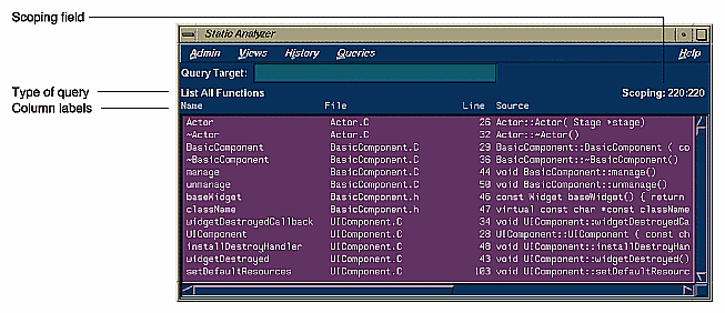
Text View's arrangement of information within each element line depends on the query type. The left field always lists the type of element you searched for; fields to its right show the location of that element and, if applicable, the contents of the source code line where it's located. For example, Text View shows the results of a function query with the function name in the first field, the filename where the function is located in the second field, the line number of the source code line where the function is defined in the next field, and the text of the line in the last field. For class queries, Text View shows any superclasses of returned classes, and for method queries, it shows the class where each method is defined.
Use the horizontal and vertical scroll bars to scroll left and right to see the full contents of long lines or up and down to work through long lists of elements respectively. To see more information at one time, you can enlarge the Static Analyzer window by dragging a corner.
To see the source code listing where an element occurs, you can double-click any element line to open the Source View window. It displays the selected element in the middle of the window, surrounded by adjacent code.
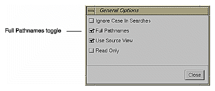
Text View normally shows filenames in the query results area as short base names. If you want to see the directory as well as the filename (or at least as full a pathname as the Static Analyzer can find), turn on the Full Pathnames option: Choose "General Options" from the Admin menu to open the General Options dialog box shown in Figure 5-2, then click the Full Pathnames button to turn on the option. Click the Close button to close the dialog box.
To return to base filenames, reopen the General Options dialog box and turn off the Full Pathnames option.
The Static Analyzer normally presents elements in the order in which they appear within each file of the fileset. To sort the elements in alphanumerical order by a single field, click the field you want within any element line, then choose "Sort" from the Admin menu. The Static Analyzer sorts the elements in ascending order by that field.
Call Tree View is designed to display functions and the static calls between them in a graphic tree form. Because it's intended for functions, it shows results only for function queries, not for other types of queries such as file and class queries. A line of text above the query results area identifies the last type of query made and shows the extent of Scope Manager reductions.
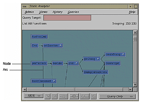
To use Call Tree View (shown in Figure 5-3), choose "Call Tree View" from the Views menu. It presents each function in the query results area as a node, a small movable box labeled with the function name, and each function call as an arc, an arrow drawn from the calling function to the called function. Because the function relationships are presented in a tree structure, higher-level functions normally appear on the left side of the window. They call lower-level functions located farther to the right.
The Static Analyzer graph view control panel (shown in Figure 5-4) below the query results area offers a set of controls that you can use to change the view. They help you see query results in the form most useful to you.
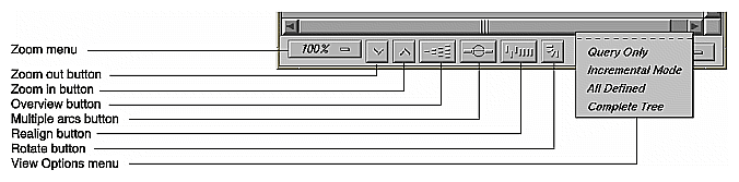
To change the scale of the call tree in the query results area to see more or less of the tree at one time, use the zoom controls: the Zoom menu and the Zoom In and Zoom Out buttons. If the tree you're viewing doesn't fit entirely within the boundaries of the query results area, you can view other parts of the tree by using the scroll bars or clicking the Overview button and navigating in the Overview window. By default, Call Tree View shows only a single arc between two functions, even if the calling function calls more than once. To see multiple calls between functions in the call tree, click the Multiple Arcs button. After maneuvering nodes, you can return them to their default positions by clicking the Realign button. The Static Analyzer's default tree orientation is horizontal; the tree grows from left to right. To see vertical tree orientation, that is, top-down (or to toggle back to horizontal), click the Rotate button.
Call Tree View allows you to directly manipulate nodes and arcs in the query results area. You can hide, reveal, and rearrange nodes, and you can select a node or an arc to view either a function or a function call in the Source View window.
For more information on the graph controls and node/arc manipulation, see Appendix A, "Using Graphical Views," in the ProDev WorkShop Overview.
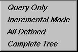
The View Options menu (at the lower right of the Call Tree View window) has four view selections that change the number of nodes you see in the query results area and change the way query results are cleared between queries (see Figure 5-5). To open the menu, move the pointer over it and hold the left mouse button down. Drag up or down to the selection you want, then release the button. The selections are:
 | Caution: The Complete Tree selection can easily create unmanageably large trees for even small programs, so use it with care. |
To view a function definition in Call Tree View, either select the function's node and choose "Edit Selected Item" from the Admin menu, or double-click the function's node. The Source View window opens with the beginning of the function definition highlighted amid surrounding code.
Call Tree View offers a Source View function not available in Text View: You can view a function call by double-clicking an arc that connects two functions. The Source View window shows the line of code (listed within the calling function) that calls the called function. You can get the same results by selecting an arc and then choosing "Edit Selected Item" from the Admin menu.
This tutorial traces function calls in Call Tree View using the "Incremental Mode" and "All Defined" viewing options. It first goes from higher- to lower-level functions using queries, and then returns to higher-level functions by showing parent nodes using the Node menu.
Move to the demo directory jello:
cd /usr/demos/WorkShop/jello
Make sure that no fileset and cross-reference files exist in the directory, so that the Static Analyzer will create its own standard default files:
rm cvstatic.*
Start the Static Analyzer:
cvstatic &
Select "Edit Fileset" from the Admin menu and move the jello.c file into the Scanner Fileset field using the Move Files Scanner button. Click OK.
This creates the fileset for this tutorial.
Choose "Call Tree View" from the Views menu to put the Static Analyzer in Call Tree View.
Choose "Incremental Mode" from the View Options menu on the bottom right side of the control panel to turn on the "Incremental Mode" view option.
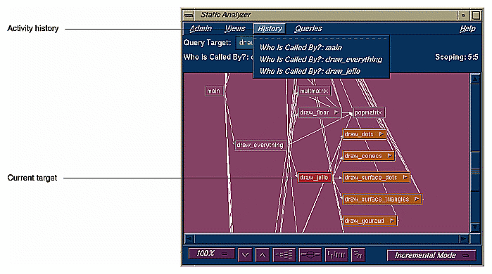
Move the pointer into the Query Target field and type main.
Choose "Who Is Called By" from the "Functions" submenu of the Query menu to find the functions that main() calls.
The Static Analyzer displays a node named main on the left side of the query results area, which displays in the target color for this scheme. It's connected by arcs to a set of lower-order function nodes to the right, all in the result color.
Drag the vertical scroll bar of the query results area down until you see the draw_everything node, then click on it to select it.
draw_everything appears in the Query Target field.
Move the pointer into the Query Target field, then press <Enter>.
The Static Analyzer repeats its last query using the new target and returns draw_everything as a target node with several result nodes to its right. The nodes from the previous query—main and its other children—still appear in the query results area in non-query color.
Select the result node draw_jello, move the pointer into the Query Target field, and press <Enter> to search for all functions called by draw_jello().
The Static Analyzer returns draw_jello as a target node with result nodes to its right as shown in Figure 5-6. The nodes from the two previous queries are still in the query results area.
Choose "15%" from the Zoom menu to set scaling to 15%.
The call tree reduces in size so that you can see all of the full call tree, although the function names are too small to be readable.
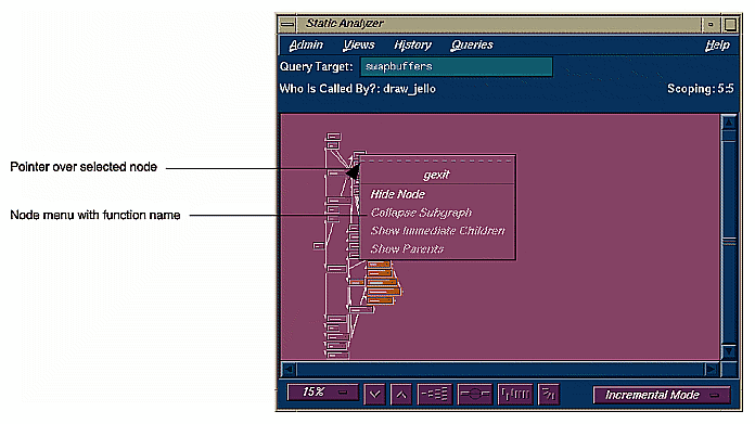
Hold down the right mouse button over any node in the tree.
The corresponding node menu displays, and the name of the function appears at the top of the menu. Using this method, you can see a large part of a tree and orient yourself by displaying the node menus (see Figure 5-7).
Click a node towards the top of the call tree and choose 100% from the Zoom menu.
This returns you to viewing at 100% and demonstrates one technique for navigating around a large call tree.
Class Tree View, which you set by choosing "Class Tree View" from the Views menu, displays a class inheritance tree containing the classes found in C++ files in the fileset. It's not intended for nonclass elements, and it won't show the results of function, file, and method queries, for example.
Class Tree View looks almost identical to Call Tree View. It includes a line of text above the query results area that lists the last query and the extent of Results Filter reductions; it shows elements in the query results area using nodes and arcs; it offers a control panel to change the view in the query results area. The main difference is that each node in Class Tree View represents a class instead of a function, and each arc shows inheritance instead of a function call. Class trees in horizontal orientation move from superclasses on the left to subclasses on the right.
When you make class queries in Class Tree View, the Static Analyzer uses colors in the same way that it does in Call Tree View: target color to mark target nodes, results color to mark result nodes, and non-query color to mark nodes not returned by the last query. The view controls also work the same way, with one minor variation. The Multiple Arcs button has no effect because no multiple inheritances exist in a class tree.
The selections in the Node and the Selected Node menus work the same way they do in Call Tree View, working through parents and children of existing nodes, but they follow class inheritance instead of a chain of function calls. Using the Source View window in Class Tree View has one minor difference: you can double-click a node to view source code for a class, but you can't double-click an arc to see an inheritance.
 | Note: The Browser lets you gather additional information on the structure, hierarchy, and method interactions of each C++ class in your application or library. |
File Dependency View, which you set by choosing "File Dependency View" from the Views menu, displays the include relationships between files in the fileset. File Dependency View is similar to Class Tree View and offers the same controls, colors, and menus. The main difference is that each node in this view represents a file in the fileset instead of a function, and each arc shows the inclusion of one file by another. An arc leads from the including file to the included file.
Although File Dependency View displays only files, it can provide useful information when used in conjunction with other types of queries. For example, if File Dependency View is displayed and you select "Where Used" from the "Function" submenu, those files containing the specified function will be highlighted.
File Dependency View is particularly useful when you are analyzing Ada source files; it shows you the dependency between packages. If you double-click arcs in this view, you can see where packages are imported using the with command and also definitions where packages are brought in.
An include tree in horizontal orientation places including files on the left and included files on the right. If you use selections from the Node and Selected Node menus to work through parents and children of existing nodes, you follow include relationships. A child of a node is a file included by that node; a parent of the node is a file that includes that node.
The Results Filter is a view tool that works in all of the Static Analyzer's views; it filters the view to show you a subset of all the results returned by a query. The Results Filter filters only the view of query results, not the results themselves. For example, if a function query returns 18 functions and the Results Filter is set to filter out 5 of them, the query results area shows only 13 functions. The Static Analyzer, however, retains the full 18 functions returned by the query; it simply hides the 5 functions filtered by the Results Filter. If you turn off all filters in the Results Filter, you then see the full 18 functions in the query results area.
When the Results Filter is set to filter, its filters remain turned on to affect the view of any future queries you make. For example, if the Results Filter is set to filter out all elements contained in header files, it does so for all queries that follow. It removes variables found in header files from a "List All Global Variables" query, and it removes header files from a "List All Files" query. You must turn off the filters if you want to see the full results of a query.
The Scoping line, located just above the right corner of the query results area, tells the extent of any filtering performed by the Results Filter. It lists two numbers separated by a colon: the first is the number of elements returned after filtering, the second is the full number of elements returned by the query. For example,
Scoping: 78:154 |
tells you that 154 elements were returned by the current query, and after filtering, the Results Filter shows 78 of them in the query results area.
To open the Results Filter window shown in Figure 5-8, choose "Results Filter" from the Admin menu.
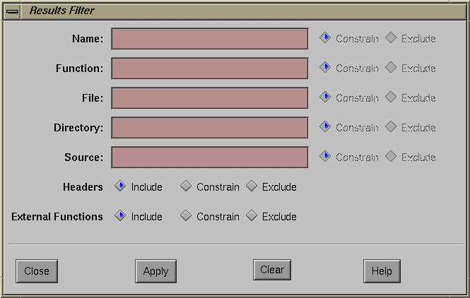
The Results Filter has seven different scope filters. The first five filters provide fields in which you can enter regular expressions, which allow you to specify a literal string of characters or a wild card expression that matches a set of strings. The last two filters require specific files and functions. The filters are:
Although the first five scope filters work using fields in Text View, their results are the same in tree views such as Call Tree View. They sort by invisible criteria in these views. For example, you can sort with the Source scope filter in Call Tree View, even though Call Tree View doesn't show the Source field for each function it displays.
To filter using the first five scope filters, enter a regular expression in the appropriate text area, and then click on either the Constrain or Exclude button following the text area. Constrain filters elements so that only those that match the regular expression in the appropriate field are displayed in the query results area. Exclude filters elements so that elements that match the regular expression in the appropriate field aren't displayed in the query results. For example, if you enter jello.c in the File scope filter and click the Constrain button, the Static Analyzer displays only elements found in the file jello.c.
To turn off filtering by any one of these five filters, delete all text from its text area.
The Headers scope filter allows three options:
| Include |
| |
| Constrain |
| |
| Exclude |
|
The External Functions scope filter also allows three options:
| Include |
| |
| Constrain |
| |
| Exclude |
|
To turn off filtering by either of these two filters, click their Include button.
You can use results filters singly or in combination to limit the elements you see to a very specific subset of the query results. For example, you can set the File filter to show only elements found in the file jello.c. You can then further refine the filtering by setting the Function filter to show only elements found in the function draw_everything(). The Static Analyzer combines these two filters to show only elements found in the function draw_everything(), which is contained in the file jello.c.
The Results Filter window displays a row of four buttons across the bottom of the window:
| Apply |
| |
| Clear |
| |
| Close |
| |
| Help |
|
This tutorial uses the Results Filter to view, in Text View, selected methods in a fileset of C++ files. It first filters the methods by file and then filters them further by a string found within each method's source code line.
Move to the demo directory bounce:
cd /usr/demos/WorkShop/bounce
Make sure that no fileset and cross-reference files exist in the directory so that the Static Analyzer will create its own standard default files:
rm cvstatic.*
Start the Static Analyzer:
cvstatic &
Use the Fileset Editor to create a fileset for bounce. If you need help, refer to "Tutorial 1: Applying the Static Analyzer to Scanned Files"
Choose "List All Methods" from the Methods submenu of the Queries menu.
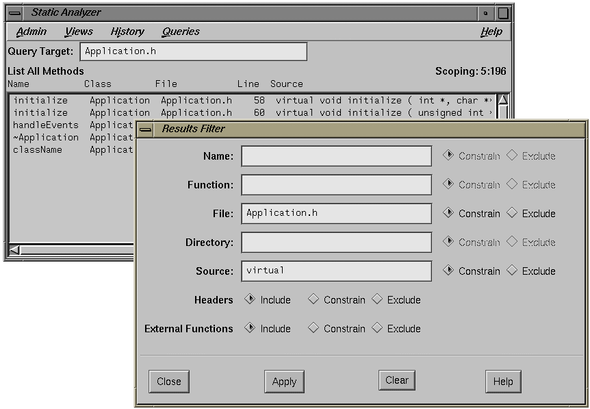
The Static Analyzer displays all methods found in the fileset. It uses Text View. The Scoping field reads 196:196, which means that all 196 elements returned by the query are displayed in the query results area. Your version of bounce may be slightly different.
Choose "Results Filter" from the Admin menu to open the Results Filter window. When it appears, drag it from on top of the Static Analyzer window so that you can see the query results area.
Move the pointer to the File field in the Results Filter window, type Application.h and click the Apply button.
The Static Analyzer shows only the methods found in the file Application.h. The Scoping field shows 16:196, which means that you see only 16 elements of the 196 returned by the current query.
Move the pointer to the Source field, type virtual, and click the Apply button.
The Static Analyzer further filters the view as shown in Figure 5-9, showing only the methods found in the file Application.h, which include the string "virtual" in their source code line. The Scoping field shows 5:196.
Click the Clear button.
The Static Analyzer clears all text fields and turns off all Results Filter filtering. All elements of the recent query return to the query results area, and the Scoping field shows 196:196.
Click the Close button to close the Results Filter window.