This chapter describes the support provided for writing parallel programs on the Origin series of computers. It assumes that you are familiar with basic parallel constructs. For more information about parallel constructs, see Chapter 5, “OpenMP Multiprocessing Directives”.
Topics covered in this chapter include:
performance tuning, “Performance Tuning of Parallel Programs on Origin series”
data distribution directives, “Data Distribution Directives”
nested DOACROSS directive, “Nested DOACROSS Directive”
affinity scheduling, “Affinity Scheduling”
processor topology, “Specifying Processor Topology With the ONTO Clause”
types of data distribution, “Types of Data Distribution”
environment variables and compile-time options, “Optional Environment Variables and Compile-Time Options ”
examples, “Examples”
A subset of the mechanisms described in this chapter are supported for C and C++, and are described in the C Language Reference Manual. You can find additional information on parallel programming in Topics in IRIX Programming.
 | Note: The multiprocessing features described in this chapter require support from the MP run-time library (libmp). IRIX operating system versions 6.3 (and above) are automatically shipped with this new library. If you wish to access these features on a machine running IRIX 6.2, contact your local Silicon Graphics service provider or SGI Customer Support (1-800-800-4744) for libmp. |
The Origin series provides cache-coherent, shared memory in the hardware. Memory is physically distributed across processors. Consequently, references to locations in the remote memory of another processor take substantially longer (by a factor of two or more) to complete than references to locations in local memory. This can severely affect the performance of programs that suffer from a large number of cache misses. Figure 6-1, shows a simplified version of the Origin series memory hierarchy.
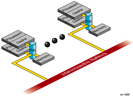
To obtain good performance in such programs, it is important to schedule computation and distribute data across the underlying processors and memory modules, so that most cache misses are satisfied from local rather than remote memory. The primary goal of the programming support, therefore, is to enable user control over data placement and computation scheduling.
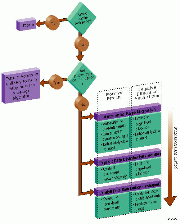
Cache behavior continues to be the largest single factor affecting performance, and programs with good cache behavior usually have little need for explicit data placement. In programs with high cache misses, if the misses correspond to true data communication between processors, then data placement is unlikely to help. In these cases, it may be necessary to redesign the algorithm to reduce inter-processor communication. Figure 6-2, shows this scenario.
If the misses are to data that is referenced primarily by a single processor, data placement may be able to convert remote references to local references, thereby reducing the latency of the miss. The possible options for data placement are automatic page migration or explicit data distribution, either regular or reshaped (both of these are described in “Regular Data Distribution”, and “Data Distribution With Reshaping”). The differences between these choices are shown in Figure 6-2.
Automatic page migration requires no user intervention and is based on the run-time cache miss behavior of the program. It can therefore adjust to dynamic changes in the reference patterns. However, the page migration heuristics are deliberately conservative, and may be slow to react to changes in the references patterns. They are also limited to performing page-level allocation of data.
Regular data distribution (performing just page-level placement of the array) is also limited to page-level allocation, but is useful when the page migration heuristics are slow and the desired distribution is known to the programmer.
Finally, reshaped data distribution changes the layout of the array thereby overcoming the page-level allocation constraints; however, it is useful only if a data structure has the same (static) distribution for the duration of the program. Given these differences, it may be necessary to use each of these options for different data structures in the same program.
For a given data structure in the program, you can choose from the options described above based on the following criteria:
If the program repeatedly references the data structure and benefits from reuse in the cache, then data placement is not needed.
If the program incurs a large number of cache misses on the data structure, then you should identify the desired distribution in the array dimensions (such as BLOCK or CYCLIC, described in “Data Distribution Directives”,) based on the desired parallelism in the program. For example, the code below suggests a distribution of A(BLOCK, *):
c$doacross
do i=2,n
  do j=2,n
    A(i,j) = 3*i + 4*j + A(i, j-1)
  enddo
enddo
Whereas, the next code segment suggests a distribution of A(*, BLOCK):
do i=2,n
c$doacross
  do j=2,n
    A(i,j) = 3*i + 4*j + A(i-1, j)
  enddo
enddo
After identifying the desired distribution, you can select either regular and reshaped distribution based on the size of an individual processor's portion of the distributed array. Regular distribution is useful only if each processor's portion is substantially larger than the page-size in the underlying system (16KBytes on the Origin2000). Otherwise regular distribution is unlikely to be useful, and you should use distribute_reshape, where the compiler changes the layout of the array to overcome page-level constraints.
For example, consider the following code:
real*8 A(m, n) c$distribute A(BLOCK, *) |
In this example, the size of each processor's portion is approximately m/P elements (8*(m/P) bytes), where P is the number of processors. If m is 1000,000 then each processor's portion is likely to exceed a page and regular distribution is sufficient. If instead m is 10,000 then distribute_reshape is required to obtain the desired distribution.
In contrast, consider the following distribution:
c$distribute A(*, BLOCK) |
In this example, the size of each processor's portion is approximately (m*n)/P elements (8*(m*n)/P bytes). So if n is 100 (for instance), regular distribution may be sufficient even if m is only 10,000.
As this example illustrates, distributing the outer dimensions of an array increases the size of an individual processor's portion (favoring regular distribution), whereas distributing the inner dimensions is more likely to require reshaped distribution.
Finally, the IRIX operating system on Origin2000 follows a default "first-touch" page-allocation policy; that is, each page is allocated from the local memory of the processor that incurs a page-fault on that page. Therefore, in programs where the array is initialized (and consequently first referenced) in parallel, even a regular distribution directive may not be necessary, because the underlying pages are allocated from the desired memory location automatically due to the first-touch policy.
The programming support consists of extensions to the existing MIPSpro Auto-Parallelizing Option (APO)/C directives/pragmas. Table 6-1, summarizes the new directives. Like the other APO/C directives, these new directives are ignored except under multiprocessor compilation using the -mp option.
Table 6-1. Summary of Directives
Directive | Description |
|---|---|
c$distribute A (dist, dist) | Data distribution. dist can be one of BLOCK, CYCLIC, CYCLIC(<expr>), or * . CYCLIC by itself implies a chunk size of 1. For performance reasons, CYCLIC(3) and CYCLIC(k) (where k has a run-time value of 3), may be incompatible when passing a reshaped array as a parameter to another routine. |
c$redistribute A(dist, dist) | Dynamic data redistribution |
c$dynamic A | Redistributable annotation |
c$distribute_reshape B(<dist>) | Data distribution with reshaping |
c*$*fill_symbol, c*$*align_symbol | Pad and align variables within pages of memory and cachelines. See the MIPSpro Compiling and Performance Tuning Guide. |
c$page_place (addr, sz, thread) | Explicit placement of data |
c$doacross affinity (i) = data (A(i)) | Data-affinity scheduling |
c$doacross affinity (i) = thread (expr) | Thread-affinity scheduling |
c$doacross nest (i,j) | Nested doacross |
The data distribution directives and doacross nest directive have an optional ONTO clause (described in “Specifying Processor Topology With the ONTO Clause”,) to control the partitioning of processors across multiple dimensions.
The data distribution directives allow you to specify High Performance Fortran-like distributions for array data structures. For irregular data structures, directives are provided to explicitly place data directly on a specific processor.
The distribute, dynamic, and distribute_reshape directives are declarations that must be specified in the declaration part of the program, along with the array declaration. The redistribute directive is an executable statement and can appear in any executable portion of the program.
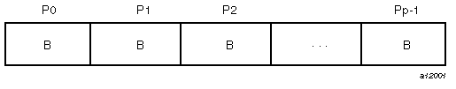
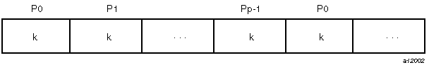
You can specify a data distribution directive for any local, global, or common-block array. Each dimension of a multi-dimensional array can be independently distributed. The possible distribution types for an array dimension are BLOCK, CYCLIC (expr), and * (asterisk not distributed). (A CYCLIC distribution with a chunk size that is either greater than 1 or is determined at runtime is sometimes also called BLOCK-CYCLIC.)
A BLOCK distribution partitions the elements of the dimension of size N into P blocks (one per processor), with each block of size B = ceiling (N/P).
A CYCLIC(k) distribution partitions the elements of the dimension into pieces of size k each, and distributes them sequentially across the processors.
A distributed array is distributed across all of the processors being used in that particular execution of the program, as determined by the MP_SET_NUMTHREADS environment variable. If a distributed array is distributed in more than one dimension, then by default the processors are apportioned as equally as possible across each distributed dimension. For instance, if an array has two distributed dimensions, then an execution with 16 processors assigns 4 processors to each dimension (4 x 4=16), whereas an execution with 8 processors assigns 4 processors to the first dimension and 2 processors to the second dimension. You can override this default and explicitly control the number of processors in each dimension using the ONTO clause along with a data distribution directive.
The nested doacross directive allows you to exploit nested concurrency in a limited manner. Although true nested parallelism is not supported, you can exploit parallelism across iterations of a perfectly nested loop-nest. For example:
c$doacross nest(i, j)
do i = 1, n
   do j = 1, m
      A(i,j) = 0
   enddo
enddo |
This directive specifies that the entire set of iterations across the (i, j) loops can be executed concurrently. The restriction is that the do i and do j loops must be perfectly nested, that is, no code is allowed between either the do i and do j statements or the enddo i and enddo j statements. You can also supply the nest clause with the PCF pdo directive.
The existing clauses such as LOCAL and SHARED behave as before. You can combine a nested doacross with an affinity clause (as shown below), or with a schedtype of simple or interleaved (dynamic and gss are not currently supported). The default is simple scheduling, except when accessing reshaped arrays (see “Affinity Scheduling” for information about scheduling).
c$doacross nest(i, j) affinity(i,j) = data(A(i,j))
do i = 2, n-1
   do j = 2, m-1
      A(i,j) = A(i,j) + i*j
   enddo
enddo |
The goal of affinity scheduling is to control the mapping of iterations of a parallel loop for execution onto the underlying threads. Specify affinity scheduling with an additional clause to a doacross directive. An affinity clause, if supplied, overrides the SCHEDTYPE clause.
The following code shows an example of data affinity:
c$distribute A(block) c$doacross affinity(i) = data(A(a*i+b)) do i = 1, n A(a*i+b) = 0 enddo |
The multiplier for the loop index variable (a) and the constant term (b) must both be literal constants, with a greater than zero.
The effect of this clause is to distribute the iterations of the parallel loop to match the data distribution specified for the array A, such that iteration i is executed on the processor that owns element A(a*i+b) based on the distribution for A. The iterations are scheduled based on the specified distribution, and are not affected by the actual underlying data-distribution (which may differ at page boundaries, for example).
In case of a multi-dimensional array, affinity is provided for the dimension that contains the loop-index variable. The loop-index variable cannot appear in more than one dimension in an affinity directive. For example:
c$distribute A (block, cyclic(1))
c$doacross affinity (i) = data (A(i+3, j))
do i = 1,n
  do j = 1,n
    A(i+3, j) = A(i+3,j-1)
  enddo
enddo |
In this example, the loop is scheduled based on the block-distribution of the first dimension. Information about doacross is in “Nested DOACROSS Directive”. The affinity clause is also available with the PCF pdo directive.
The default schedtype for parallel loops is simple. However, under -O3 compilation, level loops that reference reshaped arrays default to data-affinity scheduling for the most frequently accessed reshaped array in the loop (chosen heuristically by the compiler). To obtain simple scheduling even at -O3, you can explicitly specify the schedtype on the parallel loop.
Data affinity for loops with non-unit stride can sometimes result in non-linear affinity expressions. In such situations the compiler issues a warning, ignores the affinity clause, and defaults to simple scheduling.
By default, the compiler assumes that a distributed array is not dynamically redistributed, and directly schedules a parallel loop for the specified data affinity. In contrast, a redistributed array can have multiple possible distributions, and data affinity for a redistributed array must be implemented in the run-time system based on the particular distribution.
However, the compiler does not know if an array is redistributed, because the array may be redistributed in another function (possibly even in another file). Therefore, you must explicitly specify the c$dynamic declaration for redistributed arrays. This directive is required only in those functions that contain a doacross loop with data affinity for that array (see “Nested DOACROSS Directive”, for additional information). This informs the compiler that the array can be dynamically redistributed. Data affinity for such arrays is implemented through a run-time lookup.
Implementing data affinity through a run-time lookup incurs some extra overhead compared to a direct compile-time implementation. You can avoid this overhead when a subroutine contains data affinity for a redistributed array and the distribution of the array for the entire duration of that subroutine is known. In this situation, you can supply the c$distribute directive with the particular distribution and omit the c$dynamic directive.
By default, the compiler assumes that a distributed array is not redistributed at runtime. As a result, the distribution is known at compile time, and data affinity for the array can be implemented directly by the compiler. In contrast,because a redistributed array can have multiple possible distributions at runtime, data affinity for a redistributed array is implemented in the run-time system based on the distribution at runtime, incurring extra run-time overhead.
If an array is redistributed in the program, then you can explicitly specify a c$dynamic directive for that array. The only effect of the c$dynamic directive is to implement data affinity for that array at runtime rather than at compile time. If you know an array has a specified distribution throughout the duration of a subroutine, then you do not have to supply the c$dynamic directive. The result is more efficient compile time affinity scheduling.
Because reshaped arrays cannot be dynamically redistributed, this is an issue only for regular data distribution.
You can supply a c$distribute directive on a formal parameter, thereby specifying the distribution on the incoming actual parameter. If different calls to the subroutine have parameters with different distributions, then you can omit the c$distribute directive on the formal parameter; data affinity loops in that subroutine are automatically implemented through a run-time lookup of the distribution. This is permissible only for regular data distribution. For reshaped array parameters, the distribution must be fully specified on the formal parameter.
Similar to data affinity, you can specify thread affinity as an additional clause on a doacross directive (see “Nested DOACROSS Directive”, for details). The syntax for thread affinity is as follows:
c$doacross affinity (i) = thread(expr) |
The effect of this directive is to execute iteration i on the thread number given by the user-supplied expression (modulo the number of threads). Because the threads may need to evaluate this expression in each iteration of the loop, the variables used in the expression (other than the loop induction variable) must be declared shared and must not be modified during the execution of the loop. Violating these rules can lead to incorrect results.
If the expression does not depend on the loop induction variable, then all iterations will execute on the same thread and will not benefit from parallel execution.
This clause allows you to specify the processor topology when two (or more) dimensions of processors are required. For instance, if an array is distributed in two dimensions, then you can use the ONTO clause to specify how to partition the processors across the distributed dimensions. Or, in a nested doacross with two or more nested loops, use the ONTO clause to specify the partitioning of processors across the multiple parallel loops. The ONTO clause is also available with the PCF pdo directive.
For example:
C Assign processor in the ratio
C 1:2 to the two dimension
real*8 A (100, 200)
c$distribute A (block, block) onto (1, 2)

C Use 2 processors in the do-i loop,
C and the remaining in the do-j loop
c$doacross nest (i, j) onto (2, *)
do i = 1, n
  do j = 1, m
       . . .
  enddo
enddo |
There are two types of data distribution: regular and reshaped. The following sections describe each of these distributions.
The regular data distribution directives try to achieve the desired distribution solely by influencing the mapping of virtual addresses to physical pages without affecting the layout of the data structure. Because the granularity of data allocation is a physical page (at least 16 Kbytes), the achieved distribution is limited by the underlying page-granularity. However, the advantages are that regular data distribution directives can be added to an existing program without any restrictions, and can be used for affinity scheduling (see “Data Affinity” for details).
Distributed arrays can be dynamically redistributed with the following statement:
c$redistribute A (block, cyclic(k)) |
The redistribute statement is an executable statement that changes the distribution "permanently" (or until another redistribute statement). It also affects subsequent affinity scheduling.
The c$dynamic directive specifies that the named array is redistributed in the program, and is useful in controlling affinity scheduling for dynamically redistributed arrays. It is discussed in “Data Affinity for Redistributed Arrays”.
Similar to regular data distribution, the reshape directive specifies the desired distribution of an array. In addition, however, the reshape directive declares that the program makes no assumptions about the storage layout of that array. The compiler performs aggressive optimizations for reshaped arrays that violate standard FORTRAN 77 layout assumptions but guarantee the desired data distribution for that array.
The reshape directive accepts the same distributions as the regular data distribution directive, but uses a different keyword, as shown below:
c$distribute_reshape A(block, cyclic(1)) |
Because the distribute_reshape directive specifies that the program does not depend on the storage layout of the reshaped array, restrictions on the arrays that can be reshaped include the following:
The distribution of a reshaped array cannot be changed dynamically (that is, there is no redistribute_reshape directive).
Initialized data cannot be reshaped.
Arrays that are explicitly allocated through alloca/malloc and accessed through pointers cannot be reshaped.
An array that is equivalenced to another array cannot be reshaped.
I/O for a reshaped array cannot be mixed with namelist I/O or a function call in the same I/O statement.
A COMMON block containing a reshaped array cannot be linked -Xlocal.

Caution: This user error is not caught by the compiler/linker.
If a reshaped array is passed as an actual parameter to a subroutine, two possible scenarios exist:
The array is passed in its entirety (call func(A) passes the entire array A, whereas call func(A(i,j)) passes a portion of A). The compiler automatically clones a copy of the called subroutine and compiles it for the incoming distribution. The actual and formal parameters must match in the number of dimensions, and the size of each dimension.
You can restrict a subroutine to accept a particular reshaped distribution on a parameter by specifying a distribute_reshape directive on the formal parameter within the subroutine. All calls to this subroutine with a mismatched distribution will lead to compile- or link-time errors.
A portion of the array can be passed as a parameter, but the callee must access only a single processor's portion. If the callee exceeds a single processor's portion, then the results are undefined. You can use intrinsics to access details about the array distribution; see the dsm(3i) reference page for more details.
Most errors in accessing reshaped arrays are caught either at compile time or at link time. These include:
Inconsistencies in reshaped arrays across COMMON blocks (including across files)
Declaring a reshaped array EQUIVALENCED to another array
Inconsistencies in reshaped distributions on actual and formal parameters
Other errors such as disallowed I/O statements involving reshaped arrays, reshaping initialized data, or reshaping dynamically allocated data
Errors such as matching the declared size of an array dimension typically are caught only at runtime. The compiler option, -MP:check_reshape=on, generates code to perform these tests at runtime. These run-time checks are not generated by default, because they incur overhead, but are useful during program development.
The run-time checks include:
Inconsistencies in array-bound declarations on each actual and formal parameter
Inconsistencies in declared bounds of a formal parameter that corresponds to a portion of a reshaped actual parameter.
The compiler transforms a reshaped array into a pointer to a "processor array." The processor array has one element per processor, with the element pointing to the portion of the array local to the corresponding processor.
Figure 6-5 shows the effect of the distribute_reshape directive with a BLOCK distribution on a 1-dimensional array. N is the size of the array dimension, P is the number of processors, and B is the block-size on each processor, ceiling = (N/P).
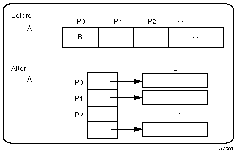
With this implementation, an array reference A(i) is transformed into a two-dimensional reference A[i/B] [i%B] (in C syntax with C dimension order), where B is the size of each block, and given by ceiling (N/P). Thus A[i/B] points to a processor's local portion of the array, and A[i/B][i%B] refers to a specific element within the local processor's portion.
A CYCLIC distribution with a chunk size of 1 is implemented as shown in Figure 6-6.
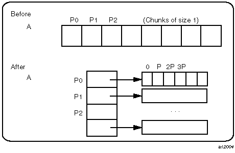
An array reference, A(i), is transformed to A[i%P] [ i/P] where P is the number of threads in that distributed dimension.
Finally, a CYCLIC distribution with a chunk size that is either a constant greater than 1 or a run-time value (also called BLOCK-CYCLIC) is implemented as Figure 6-7, shows.
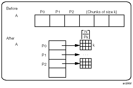
An array reference, A(i), is transformed to the three-dimensional reference A[(i/k)%P] [i/(Pk)] [i%k], where P is the total number of threads in that dimension, and k is the chunk size.
The compiler tries to optimize these divide/modulo operations out of inner loops through aggressive loop transformations such as blocking and peeling.
In summary, consider the differences between regular and reshaped data distribution. The advantage of regular distributions is that they do not impose any restrictions on the distributed arrays and can be freely applied in existing codes. Furthermore, they work well for distributions where page granularity is not a problem. For example, consider a BLOCK distribution of the columns of a two-dimensional Fortran array of size A(r, c) (column-major layout) and distribution (*, BLOCK). If the size of each processor's portion, ceiling = (c/P)*r*element_size is significantly greater than the page size (16KB on the Origin series), then regular data distribution should be effective in placing the data in the desired fashion.
However, regular data distribution is limited by page-granularity considerations. For instance, consider a (BLOCK, BLOCK) distribution of a two-dimensional array where the size of a column is much smaller than a page. Each physical page is likely to contain data belonging to multiple processors, making the data-distribution quite ineffective. (Data distribution may still be desirable from affinity-scheduling considerations, described in “Affinity Scheduling”.)
Reshaped data distribution addresses the problems of regular distributions by changing the layout of the array in memory to guarantee the desired distribution. However, because the array no longer conforms to standard FORTRAN 77 storage layout, there are restrictions on the usage of reshaped arrays.
Given both types of data distribution, you can choose between the two based on the characteristics of the particular array in an application.
For irregular data structures, you can explicitly place data in the physical memory of a particular processor using the following directive:
c$page_place (obj, size, threadnum) |
where obj is the object, size is the size of the object in bytes, and threadnum is the number of the destination processor.
This directive causes all the pages spanned by the virtual address range addr(addr+size) to be allocated from the local memory of processor number threadnum. It is an executable statement; therefore, you can use it to place either statically or dynamically allocated data.
An example of this directive is as follows:
real*8 a(100) c$page_place (a, 800, 3) |
For information on directives you can use to facilitate padding and alignment of variables within cachelines and pages of memory, see the MIPSpro Compiling and Performance Tuning Guide.
You can control various run-time features through the following optional environment variables and options. This section describes:
multiprocessing environment variables, “Multiprocessing Environment Variables ”
compile-time options, “Compile-Time Options”
The following environment variables can be used for multiprocessing:
_DSM_OFF: Disables non-uniform memory access (NUMA) specific calls (for example, to allocate pages from a particular memory).
_DSM_VERBOSE: Prints messages about parameters being used during execution.
_DSM_BARRIER: Controls the barrier implementation within the MP runtime. The accepted values are as follows:
FOP(to use the uncached operations available on the Origin platforms)
Note: Requires SGI kernel patch #1856. On Origin systems FOP achieves the best performance. SHM (to use regular shared memory). The default.
LLSC (to use LL/SC (load-linked store-conditional) operations on shared memory).
_DSM_PPM: Specifies the number of processors to use for each memory module. Must be set to an integer value; to use only one processor per memory module, set this variable to 1.
_DSM_PLACEMENT: Can be set to the following for all stack, data, and text segments:
FIRST_TOUCH (to request first-touch data placement). The default.
ROUND_ROBIN (to request round-robin data allocation across memories).
_DSM_MIGRATION: Automatic page migration is OFF by default. If set, this variable must be set to one of the following: OFF disables migration, ON enables migration except for explicitly placed data (using page_place or a data distribution directive), and ALL_ON enables migration for all data.
_DSM_MIGRATION_LEVEL: Controls the aggressiveness level of automatic page migration. Must be an integer value between 0 (most conservative, effectively disabled) and 100 (most aggressive). The default value is 100.
_DSM_WAIT: Sets the wait at a synchronization point to one of the following:
SPIN (for pure spin-waiting).
YIELD (for periodically yielding the underlying processor to another runnable job, if any). The default.
MP_SIMPLE_SCHED: Controls simple scheduling of parallel loops. This variable can be set to one of the following:
EQUAL (to distribute iterations as equally as possible across the processors).
BLOCK (to distribute iterations in a BLOCK distribution)
The default is EQUAL, unless you are using distributed arrays, in which case the default is BLOCK. The critical path (that is, the largest piece of the iteration space) is the same in either case.
MP_SUGNUMTHD: If set, this variable enables the use of dynamic threads in the multiprocessor (MP) runtime. With dynamic threads the MP runtime automatically adjusts the number of threads used for a parallel loop at runtime based on the overall system load. This feature improves the overall throughput of the system. Furthermore, by avoiding excessive concurrency, this feature can reduce delays at synchronization points within a single application.
PAGESIZE_STACK, PAGESIZE_DATA, PAGESIZE_TEXT: Specifies the desired page size in kilobytes. Must be set to an integer value.
You can find information about other environment variables on the pe_environ(5) reference page and “Specifying the Buffer Size for Direct Unformatted I/O” in Chapter 1.
Useful compile-time options include the following:
-MP:dsm=flag: flag can be ON or OFF. Default is ON.
All the data-distribution and scheduling features described in this chapter are enabled by default under -mp compilation. To disable all the DSM-specific directives (for example, distribution and affinity scheduling), compile with -MP:dsm=off.
Note: Under -mp compilation, the compiler silently generates some book-keeping information under the directory rii_files. This information is used to implement data distribution directives, as well as perform consistency checks of these directives across multiple source files. To disable the processing of the data distribution directives and not generate the rii_files, compile with the -MP:dsm=off option. -MP:clone=flag: flag can be ON or OFF. Default is ON.
The compiler automatically clones procedures that are called with reshaped arrays as parameters for the incoming distribution. However, if you have explicitly specified the distribution on all relevant formal parameters, then you can disable auto-cloning with -MP:clone=off. The consistency checking of the distribution between actual and formal parameters is not affected by this flag, and is always enabled.
-MP:check_reshape=flag: flag can be ON or OFF. Default is OFF.
Enables generation of the run-time consistency checks across procedure boundaries when passing reshaped arrays (or portions thereof) as parameters.
This section contains several examples, including:
distributing columns of a matrix, “Distributing Columns of a Matrix”
using data distribution, “Using Data Distribution and Data Affinity Scheduling”
parameter passing, “Parameter Passing”
redistributed arrays, “Redistributed Arrays”
irregular distributions, “Irregular Distributions and Thread Affinity”
The example below distributes sequentially the columns of a matrix. Such a distribution places data effectively only if the size of an individual column exceeds that of a page.
real*8 A(n, n)
C Distribute columns in cyclic fashion
c$distribute A (*, CYCLIC(1))

C Perform Gaussian elimination across columns
C The affinity clause distributes the loop iterations based
C on the column distribution of A
do i = 1, n
c$doacross affinity(j) = data(A(i,j))
   do j = i+1, n
      ... reduce column j by column i ...
     enddo
enddo |
If the columns are smaller than a page, then it may be beneficial to reshape the array. This is easily specified by changing the keyword from distribute to distribute_reshape.
In addition to overcoming size constraints as shown above, the distribute_reshape directive is useful when the desired distribution is contrary to the layout of the array. For instance, suppose you want to distribute the rows of a two-dimensional matrix. In the following example, the distribute_reshape directive overcomes the storage layout constraints to provide the desired distribution.
real*8 A(n, n)
C Distribute rows in block fashion
c$distribute_reshape A (BLOCK, *)
real*8 sum(n)
c$distribute sum(BLOCK)

C Perform sum-reduction on the elements of each row
c$doacross local(j) affinity(i) = data(A(i,j))
do i = 1,n
   do j = 1,n
      sum(i) = sum(i) + A(i,j)
   enddo
enddo |
This example demonstrates regular data distribution and data affinity. The following example, run on a 4-processor Origin2000 server, uses simple block scheduling. Processor 0 will calculate the results of the first 25,000 elements of A, processor 1 will calculate the second 25,000 elements of A, and so on. Arrays B and C are initialized using one processor; hence all of the memory pages are touched by the master processor (processor 0) and are placed in processor 0's local memory.
Using data distribution changes the placement of memory pages for arrays A, B, and C to match the data reference pattern. Thus, the code runs 33% faster on a 4-processor Origin2000 (than it would run using SMP directives without data distribution).
Without Data Distribution
   real*8 a(1000000), b(1000000)
   real*8 c(1000000)
   integer i

c$par parallel shared(a, b, c) local(i)
c$par pdo
    do i = 1, 100000
       a(i) = b(i) + c(i)
    enddo
c$par end parallel |
With Data Distribution
   real*8 a(1000000), b(1000000)
   real*8 c(1000000)
   integer i
c$distribute a(block),b(block),c(block)

c$par parallel shared(a, b, c) local(i)
c$par pdo affinity( i ) = data( a(i) )
    do i = 1, 100000
       a(i) = b(i) + c(i)
     enddo
c$par end parallel |
A distributed array can be passed as a parameter to a subroutine that has a matching declaration on the formal parameter:
real*8 A (m, n) c$distribute_reshape A (block, *) call foo (A, m, n) end subroutine foo (A, p, q) real*8 A (p, q) c$distribute_reshape A (block, *) c$doacross affinity (i) = data (A(i, j)) do i = 1, P enddo end |
Because the array is reshaped, it is required that the distribute_reshape directive in the caller and the callee match exactly. Furthermore, all calls to subroutine foo() must pass in an array with the exact same distribution.
If the array was only distributed (that is, not reshaped) in the above example, then the subroutine foo() can be called from different places with different incoming distributions. In this case, you can omit the distribution directive on the formal parameter, thereby ensuring that any data affinity within the loop is based on the distribution (at runtime) of the incoming actual parameter.
real*8 A(m, n), B (p, q) real*8 A (block, *) real*8 B (cyclic(1), *) call foo (A, m, n) call foo (B, p, q) --------------------------------------------------------- subroutine foo (X, s, t) real*8 X (s, t) c$doacross affinity (i) = data (X(i+2, j)) do i = ••• enddo |
This example shows how an array is redistributed at runtime:
subroutine bar (X, n) real*8 X(n, n) ... c$redistribute X (*, cyclic(expr)) ... end --------------------------------------------------------- subroutine foo real*8 LocalArray (1000, 1000) c$distribute LocalArray (*, BLOCK) C the call to bar() may redistribute LocalArray c$dynamic LocalArray ... call bar (LocalArray, 100) C The distribution for the following doacross C is not known statically c$doacross affinity (i) = data (A(i, j)) end |
The next example illustrates a situation where the c$dynamic directive can be optimized away. The main routine contains a local array A that is both distributed and dynamically redistributed. This array is passed as a parameter to foo() before being redistributed, and to bar() after being (possibly) redistributed. The incoming distribution for foo() is statically known; you can specify a c$distribute directive on the formal parameter, thereby obtaining more efficient static scheduling for the affinity doacross. The subroutine bar(), however, can be called with multiple distributions, requiring run-time scheduling of the affinity doacross.
program main
c$distribute A (block, *)
c$dynamic A
call foo (A)
if (x.ne.17) then
   c$redistribute A (cyclic(x), *)
endif
call bar (A)
end

subroutine foo (A)
C Incoming distribution is known to the user
c$distribute A(block, *)
c$doacross affinity (i) = data (A(i, j))
     ...
end

subroutine bar (A)
C Incoming distribution is not known statically
c$dynamic A
c$doacross affinity (i) = data (A(i, j))
     ...
end |
The example below consists of a large array that is conceptually partitioned into unequal portions, one for each processor. This array is indexed through an index array idx, which stores the starting index value and the size of each processor's portion.
real*8 A(N)
C idx ---> index array containing start index into A (idx(p, 0))
C and size (idx(p, 1)) for each processor
real*4 idx (P, 2)
c$page_place (A(idx(0, 0)), idx(0, 1)*8, 0)
c$page_place (A(idx(1, 0)), idx(1, 1)*8, 1)
c$page_place (A(idx(2, 0)), idx(2, 1)*8, 2)
...
c$doacross affinity (i) = thread(i)
do i = 0, P-1
   ... process elements on processor i...
     ...
A(idx(i, 0)) to A(idx(i,0)+idx(i,1))...
enddo |